Einstein's Equations


Describing How Mass Warps Spacetime
One of the central challenges of physics is — and has always been — to predict how things move. The earliest astronomers were really nothing more than astrologers, trying to discern when stars would appear on the horizon, or where the Sun would be found at a certain date. Eventually, this turned into true, scientific astronomy, and physicists used their laws to predict how all sorts of bodies moved through the heavens. Newton showed us that the same laws that described how planets move could also be used to predict more earth-bound things, such as how an apple falls from a tree. Modern physicists are concerned with the motions of the tiniest particles in the atoms around us, and the motions of the heaviest objects in the heavens above.
We've mentioned that geometry gives us tools to understand the motion of particles when spacetime is curved. But it doesn't say anything about why spacetime should be curved. Einstein took the tools of differential geometry, and showed us how and why spacetime curves. In doing this, he gave us very powerful tools to predict the motion of particles. To understand how these tools work will only require a little review of how to keep track of points in geometry, and the Pythagorean Theorem.
Coordinates
Suppose you want to keep track of an astronaut who is somewhere along a single line, like in our examples from the section on Relativity. You could choose a particular point — which we will call the origin — and measure how far the astronaut is from that point. If the astronaut is, for example, ten meters to the right of the origin, you might say that she is at the coordinate x=10. Ten meters to the left, and you could call it x=-10. She could even be at a fractional coordinate like x=6.78.

Of course, coordinates are just numbers that we place at each point to label that point, and to keep track of what happens at each point. We can lay those numbers down in any way we want. We might, for example, only put in one coordinate tick for every two meters. Then, if the astronaut is at a coordinate of x=5, she would still be 10 meters to the right of the origin. We say that there is a factor of proportionality which is the real distance between coordinate ticks — two, in this case. Then, if we want the actual distance, we just multiply the coordinate x by the factor of proportionality:
$$\text{distance in meters} = x \text{ coordinate} \times \text{meters per coordinate tick}$$
It's very important to remember that the real physical situation doesn't change, even if we change how we label the physical points.
Now this astronaut may want to keep track of another astronaut, but he's strayed off the coordinate axis she is on. So, she decides to create a new set of coordinates, using two dimensions to keep track of him. She takes herself as the origin and constructs two axes — one in each of the two dimensions she needs. Then, to figure out what coordinates her fellow astronaut is at, she sees how far along one axis she would need to go, then how far parallel to the other axis she would need to go. For example, our second astronaut might be six meters to the right, and eight meters up. His coordinates would be x=6 and y=8. If he were eight feet down, his coordinates would be x=6, and y=-8. We can see this in the figure below.

But now, if our first astronaut wants to get to the second, she wouldn't want to go six meters over and eight meters up; she'd want to go straight. To know how far she has to go, we need the help of an old theorem from high-school geometry.
Pythagoras's Theorem
 The Pythagorean theorem tells us the length of one side of a triangle, given the lengths of the other two sides. This is a very basic, and straightforward theorem that applies to any triangle with one right angle — that is, one angle of 90 degrees. The theorem is not very difficult to use. Suppose we have a triangle with a shortest side of 6 meters, and a second-shortest side of 8 meters. We take these numbers and square them (multiply them by themselves), giving 36 and 64 square meters. We add these together, and get 200 square meters. Now, whatever the longest side is, its square must be 100. The correct length, then, is 10 meters, since 10 squared is 100.
Using this knowledge, it's pretty easy to figure out how far apart our two astronauts are. One leg of the triangle is just the x coordinate; the other leg is the y coordinate. So, the distance between the two is given by
$$(\text{distance in meters})^2 = (x \text{ coordinate})^2 + (y \text{ coordinate})^2$$
If the coordinates measure meters, then he is 6 meters to the right and 8 meters up, so the Pythagorean Theorem tells us that he is 10 meters from the origin.
More generally, there could be a factor of proportionality to take into account, or even two — one factor for each dimension. In this case, we just have to incorporate those factors first to find the real distance in each direction, then use the Pythagorean Theorem to get the real distance from the origin. The formula in this case is just a combination of the last two formulas we've seen:
$$\begin{align}(\text{distance in meters})^2 = &((x \text{ coordinate}) \times (\text{meters per } x \text{ coordinate tick}))^2 + \\&((y \text{ coordinate}) \times (\text{meters per } y \text{ coordinate tick}))^2\end{align}$$
Basically, we've just dealt with any stretching that might happen to our grid. Of course, there's one more slight complication we'll need to deal with before we can understand Einstein's equations; some times, coordinates can be skewed, as well as stretched.
Skewed Grids and The Law of Cosines
We have already seen that curved spaces can make things complicated. For example, it's not always clear how to make a perfect square grid, like the one we assumed gave us our 2-D coordinates above. Some times, there's just no getting away from the fact coordinates might be skewed. Specifically, we might have a coordinate system where the y axis isn't perpendicular to the x axis. Instead, it might be tilted over at some angle.
We can look at this example with our two astronauts. Say the y axis is tilted over, as we see below. In this case, we would have to go farther to the right to be “under” the astronaut because when we go “up”, we have to go in the same direction as the skewed y axis. And, as a result, we would have to go farther “up” to get to him. To put some numbers to all this, say our axis is tilted by 15 degrees. Then, we'd actually have to go 8.14 meters to the right, and up 8.28 meters.

As before, we want to know how far apart the two astronauts — we want to know how long that dashed green line is. We'd like to use the Pythagorean Theorem, but that only works for right triangles — triangles with one angle of 90 degrees. Fortunately, there's a more general version that will work even in this case. All it takes is one extra term in the formula. We know the length of two sides of the triangle, and the angle between them. If we call that angle α, then the “Law of Cosines” is just like the Pythagorean theorem, except that we subtract an additional term.

Specifically, we take the normal Pythagorean Theorem, and subtract two times the length of one leg, times the length of the other leg, times the cosine of the angle between them. You might remember the cosine function here from high-school math class, written as “cos”. It takes the angle, and gives back another number, as shown below:

When α is 90 degrees, the cosine is 0, so the extra term in the Law of Cosines drops away, and it reduces to the same thing as the Pythagorean Theorem. When α is less than 90 degrees, we see that the extra term makes the side with length C smaller, which we would expect. Similarly, if α is greater than 90 degrees, the extra term makes C larger.
Now, we can apply this formula for finding the distance between the two astronauts when the coordinates are skewed by the angle α:
$$(\text{distance})^2 = (x \text{ coordinate})^2 + (y \text{ coordinate})^2 - 2 \times (x \text{ coordinate}) \times (y \text{ coordinate}) \times cos(\alpha)$$
In this case, we've already measured the two sides of the triangle to be 8.14 and 8.28 meters, and we know that the angle between them is 90 - 15 = 75 degrees. If we plug these numbers into the formula, we find that the distance squared is 100 — so the distance is 10 meters, exactly as before.
This is an important point to make: the coordinates we used to measure everything changed, but the physical situation remained the same. In particular, the distance between the two astronauts didn't change just because we skewed the coordinate grid. We could also change the coordinates in other way — by moving the origin, say, or rotating the coordinates, or any combination. But still, the physical situation (distances, for example) wouldn't change.
The Metric
When laying down a grid for coordinates, we could also combine the stretch with the skew. In general, then, we would need a formula relating distance to coordinates like
$$\begin{align}(\text{distance in meters})^2 = &[(x \text{ coordinate}) \times (\text{meters per } x \text{ coordinate tick})]^2 \\&+ [(y \text{ coordinate}) \times (\text{meters per } y \text{ coordinate tick})]^2 \\&- 2 \times [(x \text{ coordinate}) \times (\text{meters per } x \text{ coordinate tick})] \\&\times [(y \text{ coordinate}) \times (\text{meters per } y \text{ coordinate tick})] \times cos(\alpha)\end{align}$$
Obviously, this is starting to get complicated — and tiring to write out. We can save time and effort by grouping some of the terms together and writing this same formula as
$$(\text{distance in meters})^2 = g_{xx} \times (x \text{ coordinate})^2 + g_{yy} \times (y \text{ coordinate})^2 + 2 \times g_{xy} \times (x \text{ coordinate}) \times (y \text{ coordinate})$$
That is, we group those big terms together, giving them new names. Specifically, we define
$$g_{xx} = (\text{meters per }x \text{ coordinate tick})^2$$
$$g_{yy} = (\text{meters per }y \text{ coordinate tick})^2$$
$$g_{xy} = - (\text{meters per }x \text{ coordinate tick}) \times (\text{meters per }y \text{ coordinate tick}) \times cos(\alpha)$$
These three numbers we've defined — \(g_{xx}\) , \(g_{yy}\) , and \(g_{xy}\) — are very important in physics. Together, they form the metric, which relates physical distances to whatever coordinates we decide to use.
In general, the metric is just a little more complicated than the one we have shown here. First, we could be dealing with more than two dimensions. In three dimensions, we would add a z coordinate, and we would need \(g_{zz}\) , \(g_{xz}\) , and \(g_{yz}\) for the metric. We could even be working with time by adding a t coordinate. With all four dimensions, the metric involves the numbers
\(g_{xx}\) , \(g_{xy}\) , \(g_{xz}\) , \(g_{xt}\) , \(g_{yy}\) , \(g_{yz}\) , \(g_{yt}\) , \(g_{zz}\) , \(g_{zt}\) , and \(g_{tt}\) .
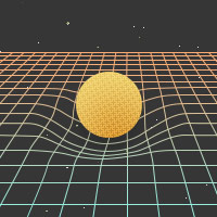
More importantly, the metric could change from place to place. If our coordinates were warped, we might have a grid that looks like our straight grid in one place, but is bent over like the second grid in another place.
It is possible to draw warped grids on a flat piece of paper (or on a flat screen, like we showed above). In this sense, we would get a warped metric in a space that is actually flat. On the other hand, it is impossible to draw a nice, straight grid in a space that is really curved. By very carefully examining exactly how the metric changes from point to point, we can tell if we've just drawn curvy coordinates in a flat space, or if we've drawn our coordinates in a truly curvy space.
Now we are getting very close to Einstein's Equations. Einstein had these warped pieces of spacetime that he needed to describe in some quantifiable way. He saw that a careful examination of the metric — and how it changes from point to point — could describe the true geometry of any spacetime, whether curved or flat, so he used it for his theory. Einstein combined certain numbers describing the metric's changes from place to place into what is now called the Einstein tensor. Just like the metric, the Einstein tensor is a set of numbers. For four-dimensional spacetime, we have
\(G_{xx}\) , \(G_{xy}\) , \(G_{xz}\) , \(G_{xt}\) , \(G_{yy}\) , \(G_{yz}\) , \(G_{yt}\) , \(G_{zz}\) , \(G_{zt}\) , and \(G_{tt}\) .
These numbers describe what is physically interesting about the geometry of spacetime. Understanding the geometry of spacetime allows us to see how particles will move, bringing us one step closer to the ultimate goal of physics. There is just one more ingredient left.
Energy, Matter, and the Curvature of Spacetime
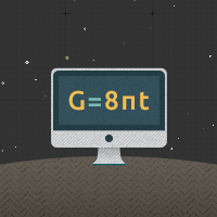
We've gotten a sneak preview of Einstein's equations before: \(G = 8πT\). The \(G\) on the left stands for the different numbers in the Einstein tensor. But, the Einstein tensor represents the geometry of spacetime, so this is what the left side really represents. We also know that the curvature of spacetime is caused by matter, so the \(T\) on the right must represent matter.
Just like \(G\), the symbol \(T\) stands for a set of numbers:
\(T_{xx}\) , \(T_{xy}\) , \(T_{xz}\) , \(T_{xt}\) , \(T_{yy}\) , \(T_{yz}\) , \(T_{yt}\) , \(T_{zz}\) , \(T_{zt}\) , and \(T_{tt}\) .
These numbers measure different things about matter. Together, they make up the Stress-Energy Tensor. Each component of this tensor has a slightly different physical interpretation:
| Pieces of the Stress-Energy Tensor | |
|---|---|
| \(T_{tt}\) | Measures how much mass there is at a point — how much density |
| \(T_{xt}\) , \(T_{yt}\) and \(T_{zt}\) | Measures how fast the matter is moving — its momentum |
| \(T_{xx}\) , \(T_{yy}\) and \(T_{zz}\) | Measures the pressure in each of the three directions |
| \(T_{xy}\) , \(T_{xz}\) and \(T_{yz}\) | Measures the stresses in the matter |
As we see from the table, things like stress, pressure, and momentum come into Einstein's equations. That is, stress, pressure, and momentum all have some effect on the warping of spacetime. This is related to Einstein's most famous equation, \(E=mc^2\), which says that energy has mass.
Warped spacetime affects how matter moves by changing its geodesics. On the other hand, Einstein's equations show us how matter — and its movement and pressures — affect the shape of spacetime. Thus, Einstein solved the fundamental problem in Physics — in principle. Of course, solving something in principle is very different from solving in practice. Finding real solutions has proven to be very difficult. Often, it is a job best left to computers.
Numerical Relativity
Four Areas of Science

Inspiration
There are more things in heaven and earth...
than are dreamt of in your philosophy.